Astronautics
MAE 146 is UC Irvine's first course in astrodynamics — the two-body problem, orbital elements, orbit transfers, Lambert's problem, and orbit perturbations. This page collects the parts of the four problem sets that I solved in code, and the final project, which was a small MATLAB toolbox and a preliminary mission analysis for a transfer to the near-Earth asteroid 65803 Didymos.
Each homework also had analytical problems — derivations, sketches, hand calculations — that are left out here; only the problems that produced a script or a figure are shown, with the code below each one.
Homework 1 — The two-body problem
The set covered the restricted two-body equations of motion, which quantities of an orbit are conserved and which vary in time, a derivation of p = a(1 − e2), a table of a, e, p and specific energy by orbit type, and a state-vector problem — eccentricity vector, energy, perigee and apogee radii, speed at a given radius, and period. One problem needed code.
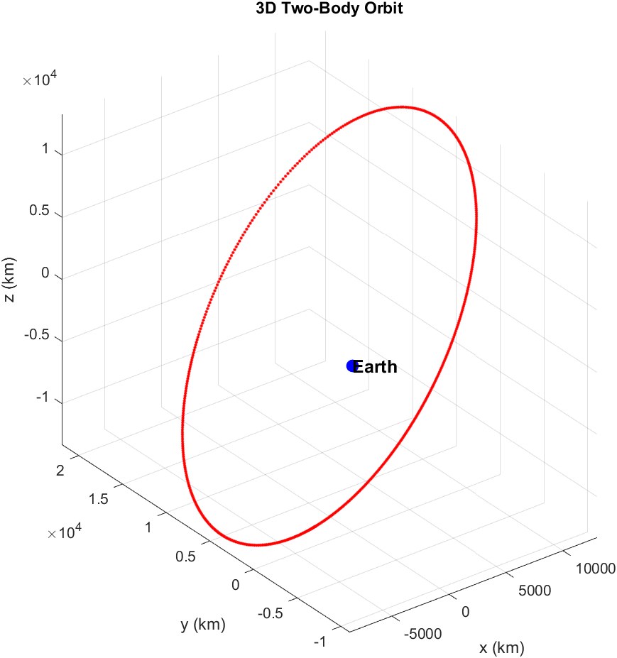
Problem 1 — Propagate and plot the orbit
Integrate ẋ = [v; −μr/‖r‖3]
with ode78 at 10−12 relative and absolute
tolerance, from r = (−8000, −6220, −7256) km
and v = (−1.5, 4.5, −4.3) km/s
over about 22 745 s, and plot the result in 3D.
%% Problem 1 - 3D Two-Body Propagation with ode78
% Aras Vakilimafakheri 2.20.26
clear; clc; close all;

% Given constants
mu = 398600.44;                 % km^3/s^2 (Earth)
tspan = [0, 22745.2295];        % s

% Initial conditions
r0 = [-8000; -6220; -7256];     % km
v0 = [-1.5; 4.5; -4.3];         % km/s
x0 = [r0; v0];                  % [r; v]

% ODE78 options (high precision)
opts = odeset('RelTol',1e-12,'AbsTol',1e-12);

% Integrate
[t, x] = ode78(@(t,x) twobody3d(t, x, mu), tspan, x0, opts);

% Extract position history
r = x(:,1:3);

%% Plot orbit in 3D
figure;
plot3(r(:,1), r(:,2), r(:,3), 'LineWidth', 1.5);
grid on; axis equal;
xlabel('x (km)'); ylabel('y (km)'); zlabel('z (km)');
title('3D Orbit Propagated with ode78');

% Optional: mark start and end
hold on;
plot3(r(1,1), r(1,2), r(1,3), 'o', 'MarkerSize', 7, 'LineWidth', 1.5);
plot3(r(end,1), r(end,2), r(end,3), 's', 'MarkerSize', 7, 'LineWidth', 1.5);
legend('Trajectory','Start','End');

function xdot = twobody3d(~, x, mu)
% x = [r; v] where r,v are 3x1
r = x(1:3);
v = x(4:6);

rnorm = norm(r);
a = -(mu / rnorm^3) * r;

xdot = [v; a];
end
Homework 2 — Orbital elements and orbit transfers
Sketching the orbital elements; converting between Cartesian state and Keplerian elements both ways; finding where an asteroid sits at perihelion; a Hohmann transfer from LEO to GEO with the plane change folded into the apogee burn, plus its propellant cost; and an ISS resupply phasing maneuver. Four of these were coded.
Problem 2 — Cartesian → Keplerian
Two states (with μ = 1) converted to {a, e, i, Ω, ω, θ} and classified by orbit type. Case (a) comes out elliptical, case (b) hyperbolic (a < 0, e > 1).
clc;
clear all;

r_vec = [0.2; 1.23; 0.6];
v_vec = [-0.8; 0.1; 0.4];
mu = 1;
r_mag = norm(r_vec);
v_mag = norm(v_vec);
h = cross(r_vec,v_vec);
e_vec = (1/mu)*(cross(v_vec,h)) - (r_vec/(r_mag));
E = 0.5*(v_mag)^2 - mu/r_mag;

a = -mu/(2*E);
e_mag = norm(e_vec);

h_z = h(3);
h_mag = norm(h);
i_rad = acos(h_z/h_mag);

i = rad2deg(i_rad);

k = [0;0;1];
holder1 = cross(k,h);
holder2 = norm(holder1);
n = holder1/holder2;

RAAN_rad = atan2(n(2),n(1));
RAAN = rad2deg(RAAN_rad);

w_rad = atan2(dot(cross(n,e_vec),h)/h_mag, dot(n,e_vec));
w = mod(rad2deg(w_rad), 360);

holder6 = dot(r_vec,v_vec);

theta_rad = atan2((h_mag*holder6)/r_mag, (h_mag^2)/r_mag - mu);
theta = mod(rad2deg(theta_rad), 360);
answerA = [a,e_mag,i,RAAN,w,theta]

clc;
clear all;

r_vec = [-2.1; 0.4; -0.6];
v_vec = [-0.1; -0.5; 1.4];
mu = 1;
r_mag = norm(r_vec);
v_mag = norm(v_vec);
h = cross(r_vec,v_vec);
e_vec = (1/mu)*(cross(v_vec,h)) - (r_vec/(r_mag));
E = 0.5*(v_mag)^2 - mu/r_mag;

a = -mu/(2*E);
e_mag = norm(e_vec);

h_z = h(3);
h_mag = norm(h);
i_rad = acos(h_z/h_mag);

i = rad2deg(i_rad);

k = [0;0;1];
holder1 = cross(k,h);
holder2 = norm(holder1);
n = holder1/holder2;

RAAN_rad = atan2(n(2),n(1));
RAAN = rad2deg(RAAN_rad);

w_rad = atan2(dot(cross(n,e_vec),h)/h_mag, dot(n,e_vec));
w = mod(rad2deg(w_rad), 360);

holder6 = dot(r_vec,v_vec);

theta_rad = atan2((h_mag*holder6)/r_mag, (h_mag^2)/r_mag - mu);
theta = mod(rad2deg(theta_rad), 360);
answerB = [a,e_mag,i,RAAN,w,theta]
answerA =   [ a        e        i        Ω        ω        θ ]
            1.5722   0.2017   35.163   37.648   345.53   63.341     (elliptical)

answerB =     -0.7580   3.8118   70.101   175.05    1.6024   341.70     (hyperbolic)
Problem 3 — Keplerian → Cartesian
The reverse map: build the perifocal position and velocity from {1.4, 0.3, 24.2°, 31°, 302°, 59°} and rotate into the inertial frame through −Ω, −i, −ω.
clc;
clear all;

vector = [1.4; 0.3; 24.2; 31; 302; 59];
mu = 1;

a = vector(1);
e = vector(2);
i = deg2rad(vector(3));
ohm = deg2rad(vector(4));
w = deg2rad(vector(5));
theta = deg2rad(vector(6));

p = a*(1 - e^2);
r = p/(1 + e*cos(theta));

r_pf = r*[cos(theta); sin(theta); 0];
v_pf = sqrt(mu/p)*[-sin(theta); e + cos(theta); 0];

R3_ohm_n = [cos(-ohm) sin(-ohm) 0; -sin(-ohm) cos(-ohm) 0; 0 0 1];
R1_i_n  = [1 0 0; 0 cos(-i) sin(-i); 0 -sin(-i) cos(-i)];
R3_w_n = [cos(-w) sin(-w) 0; -sin(-w) cos(-w) 0; 0 0 1];

holder1 = (R3_ohm_n)*(R1_i_n)*(R3_w_n);

r_vec = holder1*r_pf
v_vec = holder1*v_pf
r_vec =    0.9367   0.5833   0.0079
v_vec =   -0.3024   0.9108   0.4209
Problem 4 — Where the asteroid is closest to the Sun
For an asteroid at {2.4 AU, 0.41, 12°, 95°, 31°, 209°} the periapsis radius is a(1 − e) = 1.416 AU; placing that along the perifocal x-axis and rotating into the inertial frame gives the position vector at perihelion.
clear all;
clc;

vector = [2.4; 0.41; 12; 95; 31; 209];
mu = 1.32712e11;
AU = 149.6e6;

a = vector(1);
e = vector(2);
i = deg2rad(vector(3));
ohm = deg2rad(vector(4));
w = deg2rad(vector(5));
theta = deg2rad(vector(6));

r_p = a*(1-e)
r_p_km = r_p*AU

r_pf = r_p*[1;0;0];

R3_ohm_n = [cos(-ohm) sin(-ohm) 0; -sin(-ohm) cos(-ohm) 0; 0 0 1];
R1_i_n  = [1 0 0; 0 cos(-i) sin(-i); 0 -sin(-i) cos(-i)];
R3_w_n = [cos(-w) sin(-w) 0; -sin(-w) cos(-w) 0; 0 0 1];

holder1 = (R3_ohm_n)*(R1_i_n)*(R3_w_n);

r_vec = holder1*r_pf %[AU]

r_vec_km = r_vec*AU %[km]

%Sanity Check

norm1 = norm(r_vec)
norm2 = norm(r_vec_km)
r_p     = 1.4160 AU  (2.1183e8 km)
r_vec   = [-0.8164   1.1470   0.1516] AU
        = [-1.2214   1.7158   0.2268] x 1e8 km
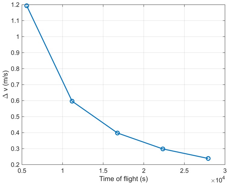
Problem 5(d) — Phasing-maneuver cost vs. number of revolutions
A resupply vehicle 10 km ahead of the ISS (427 km circular orbit) closes the gap with a phasing maneuver. Spreading the maneuver over 1–5 revolutions trades time of flight against ΔV: the longer the phasing orbit is allowed to differ from the ISS orbit by less, so the burn shrinks roughly as 1/N.
clc; clear; close all

mu = 398600;
Re = 6378;
h  = 427;
r  = Re + h;
s  = 10;

phi = s/r;
Tcirc = 2*pi*sqrt(r^3/mu);

N = 1:5;
tof = N*Tcirc;
dv  = zeros(size(N));

for k = 1:length(N)
    Tell = ((2*pi + phi/N(k))/(2*pi))*Tcirc;
    aell = (mu*(Tell/(2*pi))^2)^(1/3);
    vc   = sqrt(mu/r);
    vell = sqrt(mu*(2/r - 1/aell));
    dv(k)= 2*abs(vell - vc)*1000;
end

table(N.', tof.', dv.', 'VariableNames', {'N','Time of flight (s)','Delta v (m/s)'})

figure
plot(tof,dv,'o-','LineWidth',1.5)
grid on
xlabel('Time of flight (s)')
ylabel('\Delta v (m/s)')
N   Time of flight (s)   Delta v (m/s)
1        5.5867e+03            1.1930
2        1.1173e+04            0.5966
3        1.6760e+04            0.3977
4        2.2347e+04            0.2983
5        2.7933e+04            0.2387
Homework 3 — Kepler's problem and Gauss's problem
Two time-of-flight problems: propagating a known state forward with Kepler's equation, and solving Lambert's problem — given two position vectors and a transfer time, find the connecting orbit — with the universal-variable (Gauss) formulation.
Problem 1 — Predict the state 54 minutes later
Starting from r = (6408, 1282, −1305) km, v = (−2.2, 7.9, 2.9) km/s: reduce to orbital elements, advance the mean anomaly by nΔt over Δt = 54 min, solve Kepler's equation for the new true anomaly, and rebuild the state. The script below is the final element → state step.
clc;
clear all;

vector = [9065.74; 0.295; 21.51; 41.75; 2.406; 142.109];
mu = 398600;

a = vector(1);
e = vector(2);
i = deg2rad(vector(3));
ohm = deg2rad(vector(4));
w = deg2rad(vector(5));
theta = deg2rad(vector(6));

p = a*(1 - e^2);
r_vec = [6408; 1282; -1305];
v_vec = [-2.2; 7.9; 2.9];
r_mag = norm(r_vec);

r_pf = (p/(1 + e*cos(theta)))*[cos(theta); sin(theta); 0];
v_pf = sqrt(mu/p)*[-sin(theta); e + cos(theta); 0];

R3_ohm_n = [cos(-ohm) sin(-ohm) 0; -sin(-ohm) cos(-ohm) 0; 0 0 1];
R1_i_n  = [1 0 0; 0 cos(-i) sin(-i); 0 -sin(-i) cos(-i)];
R3_w_n = [cos(-w) sin(-w) 0; -sin(-w) cos(-w) 0; 0 0 1];

holder1 = (R3_ohm_n)*(R1_i_n)*(R3_w_n);

r_vec = holder1*r_pf
v_vec = holder1*v_pf
Problem 2 — Lambert solver, both directions
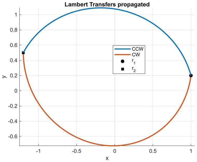
A self-contained universal-variable Lambert solver: from the transfer angle it forms the parameter A, Newton-iterates on the universal variable z (with numerically-differenced derivative) until the time-of-flight residual is under 10−8, then recovers the endpoint velocities from the Lagrange coefficients. It is run for both the short-way (counter-clockwise) and long-way (clockwise) transfers between r1 = (1, 0.2, 0.2) DU and r2 = (−1.2, 0.5, −0.03) DU over 3 TU, and each solution is propagated with the Homework 1 integrator to check it closes.
clear; close all; clc;

% Given
mu = 1;
t1 = 0;
t2 = 3.0;
dt = t2 - t1;

r1 = [ 1.0; 0.2; 0.2];
r2 = [-1.2; 0.5; -0.03];

tolLambert = 1e-8;

% Solve for CCW and CW paths
[v1_ccw, v2_ccw] = lambertUV(r1, r2, dt, mu, false, tolLambert);
[v1_cw,  v2_cw ] = lambertUV(r1, r2, dt, mu, true,  tolLambert);

disp('CCW');
disp('v1 ='); disp(v1_ccw);
disp('v2 ='); disp(v2_ccw);

disp('CW');
disp('v1 ='); disp(v1_cw);
disp('v2 ='); disp(v2_cw);

%% Propagate from HW 1
tspan = [t1 t2];
options = odeset('RelTol',1e-12,'AbsTol',1e-12);

% Intial State Vector
x0_ccw = [r1; v1_ccw];
x0_cw  = [r1; v1_cw ];

[t_ccw, x_ccw] = ode78(@(t,x) twobody3D(t,x,mu), tspan, x0_ccw, options);
[t_cw,  x_cw ] = ode78(@(t,x) twobody3D(t,x,mu), tspan, x0_cw,  options);

%% Plot
figure; hold on; grid on; axis equal;

plot3(x_ccw(:,1), x_ccw(:,2), x_ccw(:,3), 'LineWidth', 2);
plot3(x_cw(:,1),  x_cw(:,2),  x_cw(:,3),  'LineWidth', 2);

plot3(r1(1), r1(2), r1(3), 'ko', 'MarkerFaceColor','k');
plot3(r2(1), r2(2), r2(3), 'ks', 'MarkerFaceColor','k');

xlabel('x'); ylabel('y'); zlabel('z');
title('Lambert Transfers propagated');
legend('CCW','CW','r_1','r_2','Location','best');

%% Functions

function dx = twobody3D(~, x, mu)
r = x(1:3);
v = x(4:6);
rn = norm(r);
dx = [v; -(mu/rn^3)*r];
end

function [v1, v2] = lambertUV(r1, r2, dt, mu, longway, tol)
r1n = norm(r1);
r2n = norm(r2);

c = dot(r1,r2)/(r1n*r2n);
c = max(-1,min(1,c));
dnu = acos(c);
if longway
    dnu = 2*pi - dnu;
end

A = sin(dnu)*sqrt(r1n*r2n/(1 - cos(dnu)));

z = 0;                % initial guess
for k = 1:200
    [C,S] = stumpff(z);

    y = r1n + r2n + A*(z*S - 1)/sqrt(C);
    if y < 0
        z = z + 0.1;
        continue
    end

    x = sqrt(y/C);
    dtz = (x^3*S + A*sqrt(y))/sqrt(mu);

    F = dtz - dt;
    if abs(F) < tol
        break
    end

    h = 1e-5;
    [Cp,Sp] = stumpff(z+h);
    yp = r1n + r2n + A*((z+h)*Sp - 1)/sqrt(Cp);
    xp = sqrt(yp/Cp);
    dtp = (xp^3*Sp + A*sqrt(yp))/sqrt(mu);

    [Cm,Sm] = stumpff(z-h);
    ym = r1n + r2n + A*((z-h)*Sm - 1)/sqrt(Cm);
    xm = sqrt(ym/Cm);
    dtm = (xm^3*Sm + A*sqrt(ym))/sqrt(mu);

    dFdz = ( (dtp-dt) - (dtm-dt) )/(2*h);

    z = z - F/dFdz;
end


[C,S] = stumpff(z);
y = r1n + r2n + A*(z*S - 1)/sqrt(C);

f    = 1 - y/r1n;
g    = A*sqrt(y/mu);
gdot = 1 - y/r2n;

v1 = (r2 - f*r1)/g;
v2 = (gdot*r2 - r1)/g;
end

function [C,S] = stumpff(z)

if abs(z) < 1e-8
    C = 1/2; S = 1/6; return
end

if z > 0
    s = sqrt(z);
    C = (1 - cos(s))/z;
    S = (s - sin(s))/(s^3);
else
    s = sqrt(-z);
    C = (cosh(s) - 1)/(-z);
    S = (sinh(s) - s)/(s^3);
end
end
CCW    v1 = [-0.2650   0.9806   0.2403]      v2 = [-0.3800  -0.7030  -0.2539]
CW     v1 = [-0.1278  -0.9923  -0.2999]      v2 = [-0.0048   0.8076   0.2285]
Homework 4 — Interplanetary transfers and J2
Patched-conic interplanetary transfers — Earth → Venus Hohmann with hyperbolic escape and capture, a Jupiter gravity-assist turn, lunar sphere-of-influence and geosynchronous-orbit feasibility, and Sun-synchronous conditions at Mars — then ground-track matching, and a propagator for the oblateness (J2) perturbation. The propagator was the coded problem.
Problem 6 — Propagating an orbit under J2
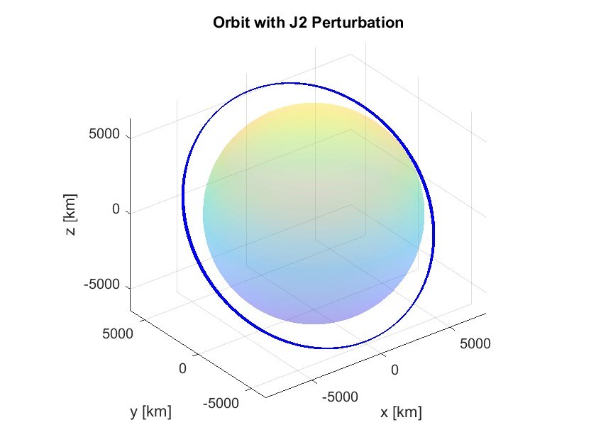
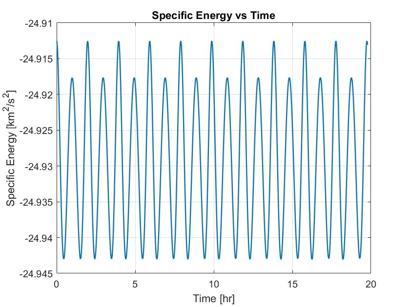
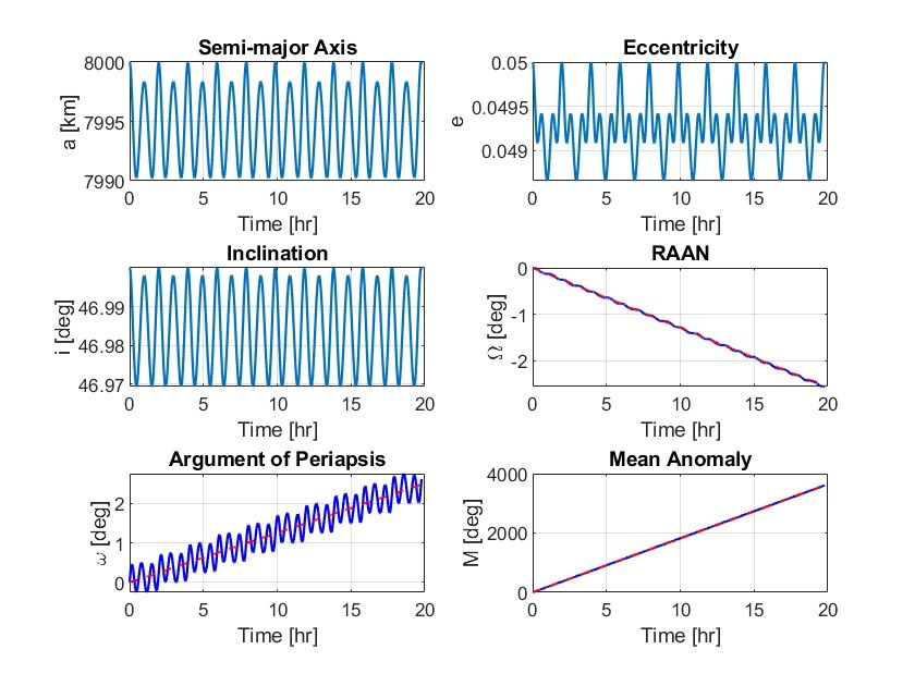
Integrate the two-body motion plus the J2 acceleration for an 8000 km, e = 0.05, i = 47° orbit over ten periods; then convert the state history back to osculating elements and overlay the secular J2 rates for Ω, ω and M. The plots show the node regressing, periapsis advancing, and the mean anomaly running slightly fast — while a, e and i only oscillate.
%% Problem 6 - J2 orbit propagation
% This script propagates an Earth orbit with J2 perturbations, then
% plots the orbit, specific energy, and osculating Keplerian elements.

clear
clc
close all

%% Define constants
mu = 398600.44;          % Earth's gravitational parameter [km^3/s^2]
J2 = 1.08263e-3;         % Earth's J2 coefficient [-]
Re = 6378.1363;          % Earth's equatorial radius [km]

%% Define initial Keplerian elements
a0  = 8000;              % semi-major axis [km]
e0  = 0.05;              % eccentricity [-]
i0  = deg2rad(47);       % inclination [rad]
Om0 = 0;                 % RAAN [rad]
w0  = 0;                 % argument of periapsis [rad]
ta0 = 0;                 % true anomaly [rad]

%% Build initial Keplerian element vector
kep0 = [a0; e0; i0; Om0; w0; ta0];

%% Convert initial Keplerian elements to Cartesian state
x0 = kep2rv(kep0, mu);   % initial state vector [r0; v0]

%% Compute the initial orbital period
T0 = 2*pi*sqrt(a0^3/mu); % orbital period [s]

%% Define the propagation time span for 10 orbital periods
tspan = linspace(0, 10*T0, 5000);

%% Set ODE solver tolerances
opts = odeset('RelTol', 1e-11, 'AbsTol', 1e-12);

%% Propagate the orbit with J2 perturbation
[t, x] = ode45(@(t,x) j2_eom(x, mu, J2, Re), tspan, x0, opts);

%% Extract position and velocity histories
r = x(:,1:3);            % position history [km]
v = x(:,4:6);            % velocity history [km/s]

%% Plot the 3D orbit
figure
plot3(r(:,1), r(:,2), r(:,3), 'b', 'LineWidth', 1.2)
hold on

%% Draw Earth as a sphere
[Xe, Ye, Ze] = sphere(50);
surf(Re*Xe, Re*Ye, Re*Ze, 'EdgeColor', 'none', 'FaceAlpha', 0.25)

%% Format the 3D orbit plot
axis equal
grid on
xlabel('x [km]')
ylabel('y [km]')
zlabel('z [km]')
title('Orbit with J2 Perturbation')

%% Compute specific orbital energy at each time step
rmag = vecnorm(r, 2, 2);             % magnitude of each position vector [km]
vmag = vecnorm(v, 2, 2);             % magnitude of each velocity vector [km/s]
energy = 0.5*vmag.^2 - mu./rmag;     % specific orbital energy [km^2/s^2]

%% Plot specific energy versus time
figure
plot(t/3600, energy, 'LineWidth', 1.2)
grid on
xlabel('Time [hr]')
ylabel('Specific Energy [km^2/s^2]')
title('Specific Energy vs Time')

%% Preallocate storage for osculating Keplerian elements
kep_hist = zeros(length(t), 6);      % each row is [a e i Om w ta]
M = zeros(length(t), 1);             % mean anomaly history [rad]

%% Convert each propagated state back to Keplerian elements
for k = 1:length(t)
    kep_hist(k,:) = rv2kep(x(k,:).', mu).';      % store osculating elements
    M(k) = ta2ma(kep_hist(k,2), kep_hist(k,6));  % convert true anomaly to mean anomaly
end

%% Extract individual element histories
a   = kep_hist(:,1);      % semi-major axis history [km]
e   = kep_hist(:,2);      % eccentricity history [-]
inc = kep_hist(:,3);      % inclination history [rad]
Om  = kep_hist(:,4);      % RAAN history [rad]
w   = kep_hist(:,5);      % argument of periapsis history [rad]
ta  = kep_hist(:,6);      % true anomaly history [rad]

%% Convert angular histories to degrees for plotting
inc_deg = rad2deg(inc);           % inclination [deg]
Om_deg  = rad2deg(unwrap(Om));    % unwrapped RAAN [deg]
w_deg   = rad2deg(unwrap(w));     % unwrapped argument of periapsis [deg]
M_deg   = rad2deg(unwrap(M));     % unwrapped mean anomaly [deg]

%% Compute secular J2 rates using the initial orbit
p0 = a0*(1 - e0^2);               % semi-latus rectum [km]
n0 = sqrt(mu/a0^3);               % mean motion [rad/s]

Om_dot = -(3/2)*J2*n0*(Re/p0)^2*cos(i0);
w_dot  =  (3/4)*J2*n0*(Re/p0)^2*(5*cos(i0)^2 - 1);
M_dot  =  n0 + (3/4)*J2*n0*(Re/p0)^2*sqrt(1 - e0^2)*(3*cos(i0)^2 - 1);

%% Build secular mean trends for overlay
Om_mean = rad2deg(Om0 + Om_dot*t);    % secular RAAN trend [deg]
w_mean  = rad2deg(w0 + w_dot*t);      % secular argument of periapsis trend [deg]
M_mean  = rad2deg(M_dot*t);           % secular mean anomaly trend [deg]

%% Plot osculating Keplerian elements
figure

subplot(3,2,1)
plot(t/3600, a, 'LineWidth', 1.1)
grid on
xlabel('Time [hr]')
ylabel('a [km]')
title('Semi-major Axis')

subplot(3,2,2)
plot(t/3600, e, 'LineWidth', 1.1)
grid on
xlabel('Time [hr]')
ylabel('e')
title('Eccentricity')

subplot(3,2,3)
plot(t/3600, inc_deg, 'LineWidth', 1.1)
grid on
xlabel('Time [hr]')
ylabel('i [deg]')
title('Inclination')

subplot(3,2,4)
plot(t/3600, Om_deg, 'b', 'LineWidth', 1.1)
hold on
plot(t/3600, Om_mean, 'r--', 'LineWidth', 1.1)
grid on
xlabel('Time [hr]')
ylabel('\Omega [deg]')
title('RAAN')

subplot(3,2,5)
plot(t/3600, w_deg, 'b', 'LineWidth', 1.1)
hold on
plot(t/3600, w_mean, 'r--', 'LineWidth', 1.1)
grid on
xlabel('Time [hr]')
ylabel('\omega [deg]')
title('Argument of Periapsis')

subplot(3,2,6)
plot(t/3600, M_deg, 'b', 'LineWidth', 1.1)
hold on
plot(t/3600, M_mean, 'r--', 'LineWidth', 1.1)
grid on
xlabel('Time [hr]')
ylabel('M [deg]')
title('Mean Anomaly')

%% J2 equations of motion
function dx = j2_eom(x, mu, J2, Re)
    % Extract position and velocity from the state vector
    r = x(1:3);
    v = x(4:6);

    % Extract Cartesian position components
    x1 = r(1);
    y1 = r(2);
    z1 = r(3);

    % Compute radius magnitude and useful repeated terms
    rmag = norm(r);
    r2 = rmag^2;
    z2 = z1^2;

    % Compute central two-body gravitational acceleration
    a2b = -mu*r/rmag^3;

    % Compute J2 perturbation acceleration coefficient
    f = 1.5*J2*mu*Re^2/rmag^5;

    % Compute J2 perturbation acceleration vector
    aJ2 = f * [x1*(5*z2/r2 - 1);
               y1*(5*z2/r2 - 1);
               z1*(5*z2/r2 - 3)];

    % Return time derivative of the state vector
    dx = [v; a2b + aJ2];
end
Final project — an astrodynamics toolbox, and a mission to Didymos
The project was built in four parts. The first three fill in a small library of routines, each checked against a provided test harness; the fourth uses them for a preliminary mission analysis.
Problems 1–3 — The toolbox
Problem 1 — rv2kep and
kep2rv, the two-way map between an inertial state and the
Keplerian elements, with the circular and equatorial edge cases handled.
Problem 2 — ta2ma / ma2ta
between true and mean anomaly (Newton on Kepler's equation), and
propagate_elliptical, which advances a state along its
ellipse by going to elements, stepping the mean anomaly, and coming
back. Problem 3 — the stumpff
functions and lambert_universal, a universal-variable
Lambert solver with an initial bracket and Newton refinement.
Problem 1 — element conversions
function kep = rv2kep(rv, MU)
% RV2KEP Converts a state vector x = [r; v] ∈ R6 in the inertial frame
% to Keplerian elements {a, e, i, Ω, ω, θ}
%
% Inputs:
%   rv = 6 by 1 inertial Cartesian state [r; v]
%         r = position vector (3x1)
%         v = velocity vector (3x1)
%   MU = Standard Gravitational Parameter
%
% Outputs:
%   kep = 6 by 1 vector of Keplerian Elements
%
    arguments (Input)
        rv (6,1) double     % cartesian vector
        MU (1,1) double     % gravitational parameter
    end

    arguments (Output)
        kep (6,1) double    % Keplerian elements vector [a; e; i; W; w; ta]
    end

    %% Extract position and velocity and compute magnitudes
    r_vec = rv(1:3);
    v_vec = rv(4:6);

    r = norm(r_vec);
    v = norm(v_vec);

    %% Compute specific angular momentum vector and magnitude
    h_vec = cross(r_vec,v_vec);
    h = norm(h_vec);

    %% Compute eccentricity vector and magnitude
    e_vec = (1/MU)*cross(v_vec, h_vec) - (r_vec/r);
    e = norm(e_vec);

    %% Compute specific orbital energy and semi-major axis
    E = 0.5*v^2 - MU/r;
    a = -MU/(2*E);

    %% Compute inclination angle
    i = acos(h_vec(3)/h);

    % Node vector
    k = [0;0;1];
    n_vec = cross(k, h_vec);
    n = norm(n_vec);

    %% Commpute right ascension of the ascending node
    if n > 1e-12
        W = atan2(n_vec(2), n_vec(1));
        W = mod(W, 2*pi);
    else
        W = 0; % if n ~ 0 then Ω is undefined, so set to zero
    end

    %% Compute argument of periapsis
    if e > 1e-10
        w = acos(dot(n_vec, e_vec)/(n*e));
        if e_vec(3) < 0
            w = (2*pi)-w;
        end
    else
        w = 0; % if e ~ 0 then ω is undefined, so set to zero
    end

    %% Commpute true anomaly
    % Quadrant is determined using the sign of r · v.
    % If the orbit is circular, periapsis is undefined,
    % so θ is measured from the node vector instead.
    if e > 1e-10
        ta = acos(dot(e_vec, r_vec)/(e*r));
        if dot(r_vec, v_vec) < 0
            ta = (2*pi)-ta;
        end
    else
        % circular
        if n > 1e-12
            ta = acos(dot(n_vec, r_vec)/(n*r));
            if r_vec(3) < 0
                ta = (2*pi)-ta;
            end
        else
            ta = 0;
        end
    end

    %% Output
    kep = [a; e; i; W; w; ta];
end
function rv = kep2rv(kep, MU)
% KEP2RV Converts Keplerian elements {a, e, i, Ω, ω, θ} to the
% corresponding inertial state vector x = [r; v] ∈ R6
%
% Inputs:
%   kep = 6 by 1 vector of Keplerian Elements
%   MU = Standard Gravitational Parameter
%
% Outputs:
%   rv = 6 by 1 inertial Cartesian state [r; v]
%         r = position vector (3x1)
%         v = velocity vector (3x1)
%
    arguments (Input)
        kep (6,1) double     % Keplerian elements vector
        MU  (1,1) double     % gravitational parameter
    end

    arguments (Output)
        rv (6,1) double    % return 6-by-1 state vector
    end

    %% Extract Keplerian elements from the input vector
    a = kep(1);     % Semi-major axis
    e = kep(2);     % Eccentricity
    i = kep(3);    % Inclination
    W = kep(4);  % RAAN
    w = kep(5);    % Argument of periapsis
    ta = kep(6);    % True anomaly

    %% Compute semi-latus rectum
    p = a*(1 - e^2);

    %% Compute radius
    r = p/(1 + e*cos(ta));

    %% Compute position and velocity in perifocal frame
    r_pf = r*[cos(ta); sin(ta); 0];
    v_pf = sqrt(MU/p)*[-sin(ta); e + cos(ta); 0];

    %% Construct rotation matrix from perifocal to inertial
    R3_ohm_n = [cos(-W) sin(-W) 0; -sin(-W) cos(-W) 0; 0 0 1];
    R1_i_n  = [1 0 0; 0 cos(-i) sin(-i); 0 -sin(-i) cos(-i)];
    R3_w_n = [cos(-w) sin(-w) 0; -sin(-w) cos(-w) 0; 0 0 1];

    Q = (R3_ohm_n)*(R1_i_n)*(R3_w_n);

    %% Convert into interial frame
    r_vec = Q*r_pf;
    v_vec = Q*v_pf;

    %% Output
    rv = [r_vec; v_vec];
end
Problem 2 — anomaly conversions and propagation
function ma = ta2ma(e, ta)
% TA2MA Converts true anomaly θ to mean anomaly M
%
% Inputs:
%   e = Eccentricity
%   ta = True Anomaly
%
% Outputs:
%   ma = Mean anomaly
%
    arguments (Input)
        e  (1,1) double     % eccentricity
        ta (1,1) double     % true anomaly
    end

    arguments (Output)
        ma (1,1) double    % mean anomaly
    end

    %% Convert true anomaly to eccentric anomaly
    cosE = (e + cos(ta)) / (1 + e*cos(ta));
    sinE = sqrt(1 - e^2) * sin(ta) / (1 + e*cos(ta));

    E = acos(cosE);

    % Quadrant correction
    if sinE < 0
        E = 2*pi - E;
    end

    %% Convert eccentric anomaly to mean anomaly
    ma = E - e*sin(E);
end
function ta = ma2ta(e, ma)
% MA2TA Converts mean anomaly M to true anomaly θ
%
% Inputs:
%   e = Eccentricity
%   ma = Mean anomaly
%
% Outputs:
%   ta = True Anomaly
%
    arguments (Input)
        e  (1,1) double     % eccentricity
        ma (1,1) double     % mean anomaly
    end

    arguments (Output)
        ta (1,1) double    % true anomaly
    end

    %% Solve Kepler's Equation for eccentric anomaly using iteration
    tol = 1e-12;
    Nmax = 50;
    E = ma;   % initial guess

    for k = 1:Nmax
        f  = E - e*sin(E) - ma;
        fp = 1 - e*cos(E);
        E  = E - f/fp;
        if abs(f) < tol
            break
        end
    end

    %% Convert eccentric anomaly to true anomaly
    cos_ta = (cos(E) - e) / (1 - e*cos(E));
    sin_ta = (sqrt(1 - e^2)*sin(E)) / (1 - e*cos(E));

    ta = acos(cos_ta);

    % Quadrant correction
    if sin_ta < 0
    ta = 2*pi - ta;
    end
end
function ta = propagate_elliptical_ta(period, e, ta0, tof)
% PROPAGATE_ELLIPTICAL_TA Computes the true anomaly after time of flight
% along a circular or elliptical orbit.
%
% Inputs:
%   Period
%   e = Eccentricity
%   ta0 = Initial true anomaly
%   tof = Time of flight
%
% Outputs:
%   ta = True anomaly after time of flight
%
    arguments (Input)
        period (1,1) double    % period
        e      (1,1) double    % eccentricity
        ta0    (1,1) double    % initial true anomaly
        tof    (1,1) double    % time of flight
    end

    arguments (Output)
        ta (1,1) double        % true anomaly after tof
    end

    assert(e < 1) % assumes elliptical orbit

    %% Convert true anomaly initial to mean anomaly via ta2ma function
    ma0 = ta2ma(e, ta0);

    %% Define Mean Motion "n" = sqrt(mu/a^3) = 2pi/period
    n = 2*pi/period;

    %% Use Kepler's Equation in time for to propgate mean anomaly forward
    ma = ma0 + n*tof;

    %% Use ma2ta with the propagted mean anomaly to find true anomaly after tof
    ta = ma2ta(e, ma);
end
function rvf = propagate_elliptical(rv, tof, MU)
% PROPAGATE_ELLIPTICAL Propagates the Cartesian state
% x(t0) = [r(t0); v(t0)] over time tof and returns the final state
% x(tof) = [r(tof); v(tof)].
%
%
% Inputs:
%   rv = 6 by 1 initial Cartesian state [r; v]
%         r = position vector (3x1)
%         v = velocity vector (3x1)
%   tof = Time of flight
%   MU = Standard gravitational parameter
%
% Outputs:
%   rvf = 6 by 1 final Cartesian state [rf; vf]
%
    arguments (Input)
        rv  (6,1) double     % initial cartesian vector
        tof (1,1) double     % time of flight
        MU  (1,1) double     % gravitational parameter
    end

    arguments (Output)
        rvf (6,1) double        % final position & velocity vector [rf; vf]
    end

    %% Convert initial state vector in the intertial frame to
    %% Keplerian Elements via rv2kep
    kep = rv2kep(rv, MU);
    a   = kep(1);   % semi-major axis
    e   = kep(2);   % eccentricity
    ta0 = kep(6);   % initial true anomaly

    assert(e < 1)   % assumes elliptical orbit

    %% Compute orbital period
    period = 2*pi*sqrt(a^3/MU);

    %% Compute the true anomaly after time of flight tof
    %% along a circular/elliptical orbit
    ta = propagate_elliptical_ta(period, e, ta0, tof);

    %% Replace true anomaly in the Keplerian element vector
    kep(6) = ta;

    %% Convert new Keplerian elements back to Cartesian state
    rvf = kep2rv(kep, MU);
end
Problem 3 — Stumpff functions and Lambert solver
function [C,S] = stumpff(z,eps)
% STUMPFF evaluates the Stumpff functions C(z) and S(z).
% Inputs:
%   z = Function input
%   eps = Tolerance for when z approaches zero
%
% Outputs:
%   C = Stumpff function C evaluated at z
%   S = Stumpff function S evaluated at z
%
    arguments (Input)
        z   (1,1) double    % function input
        eps (1,1) double    % tolerance for Stumpff functions near 0
    end

    arguments (Output)
        C (1,1) double      % Stumpff function C evaluated at z
        S (1,1) double      % Stumpff function S evaluated at z
    end

    %% Evaluate Stumpff functions based on sign of z

    if z > eps % Elliptic case = z > 0
        sqz = sqrt(z);
        C = (1 - cos(sqz)) / z;
        S = (sqz - sin(sqz)) / (sqz^3);

    elseif z < -eps  % Hyperbolic case = z < 0
        sqz = sqrt(-z);
        C = (cosh(sqz) - 1) / (-z);
        S = (sinh(sqz) - sqz) / (sqz^3);

    else % Limiting values as z approaches zero
        C = 1/2 - z/24 + z^2/720 - z^3/40320;
        S = 1/6 - z/120 + z^2/5040 - z^3/362880;
end
function [v1, v2, residual] = lambert_universal(r1, r2, tof, MU, cw, eps, tol)
% LAMBERT_UNIVERSAL Solves Lambert's problem using universal variables.
%
% Inputs:
%   r1 = Initial position vector
%   r2 = Final position vector
%   tof = Time of flight
%   MU = Standard Gravitational Parameter
%   cw = Clockwise flag
%          if cw = 0 ccw prograde transfer
%          if cw = 1 cw retrograde transfer
%   eps = Tolerance for when z approaches zero
%   tol = Tolerance for root-solving
%
% Outputs:
%   v1 = Initial velocity vector
%   v2 = Final velocity vector (3x1)
%   residual
%
    arguments (Input)
        r1  (3,1) double    % initial position vector
        r2  (3,1) double    % final position vector
        tof (1,1) double    % time of flight
        MU  (1,1) double    % gravitational parameter
        cw  (1,1) double    % whether to use clockwise path, 0 or 1
        eps (1,1) double    % tolerance for Stumpff functions near 0
        tol (1,1) double    % tolerance on root-solving
    end

    arguments (Output)
        v1 (3,1) double         % initial velocity vector
        v2 (3,1) double         % final velocity vector
        residual (1,1) double   % residual on converged root-solving problem
    end

    %% Compute magnitudes of the endpoint position vectors
   r1mag = norm(r1);
   r2mag = norm(r2);

   %% Compute transfer angle with prograde/retrograde correction
   cos_dtheta = max(-1,min(1,dot(r1,r2)/(r1mag*r2mag)));
   dtheta = acos(cos_dtheta);
   crossz = r1(1)*r2(2) - r1(2)*r2(1);           % z-component of r1 × r2
   if (cw == 0 && crossz <= 0) || (cw == 1 && crossz >= 0)
       dtheta = 2*pi - dtheta;
   end

   %% Compute Lambert Parameter
   A = sin(dtheta)*sqrt(r1mag*r2mag/(1-cos(dtheta)));
   if abs(A) < 1e-8
       error('degenerate A = 0 r1 and r2 are collinear');
   end

   % Initial bracket for Newton iteration
   z = -100;
   while tof_F(z, r1mag, r2mag, A, tof, MU, eps) < 0
       z = z + 0.1;
   end

   % Newton iteration
   nmax = 20000;  n = 0;  ratio = 1;
   while abs(ratio) > tol && n <= nmax
       n = n + 1;
       ratio = tof_F(z, r1mag, r2mag, A, tof, MU, eps) / tof_dFdz(z, r1mag, r2mag, A, eps);
       z = z - ratio;
   end

   if n >= nmax
       warning('Newton''s method did not converge within %d iterations', nmax);
   end

   residual = abs(tof_F(z, r1mag, r2mag, A, tof, MU, eps));

   %% Turning Lagrange coefficients to velocities
   [C, S] = stumpff(z, eps);
   y = r1mag + r2mag + A*(z*S - 1)/sqrt(C);
   f = 1 - y/r1mag;
   g = A*sqrt(y/MU);
   gdot = 1 - y/r2mag;

   v1 = (r2 - f*r1)/g;
   v2 = (gdot*r2 - r1)/g;
   end

   %% Local Functions
   function val = tof_F(z, r1n, r2n, A, tof, MU, eps)
       [C, S] = stumpff(z, eps);
       y = r1n + r2n + A*(z*S - 1)/sqrt(C);
       val = (y/C)^1.5 * S + A*sqrt(y) - sqrt(MU)*tof;
   end


   function val = tof_dFdz(z, r1n, r2n, A, eps)
       [C, S] = stumpff(z, eps);
       y = r1n + r2n + A*(z*S - 1)/sqrt(C);
       if z == 0
           val = sqrt(2)/40 * y^1.5 + A/8*(sqrt(y) + A/sqrt(2*y));
       else
           val = (y/C)^1.5 * (1/(2*z)*(C - 3*S/(2*C)) + 3*S^2/(4*C))  ...
           + A/8*(3*S/C*sqrt(y) + A*sqrt(C/y));
       end
   end
Problem 4 — Mission to Didymos
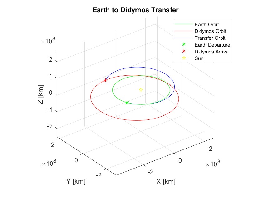
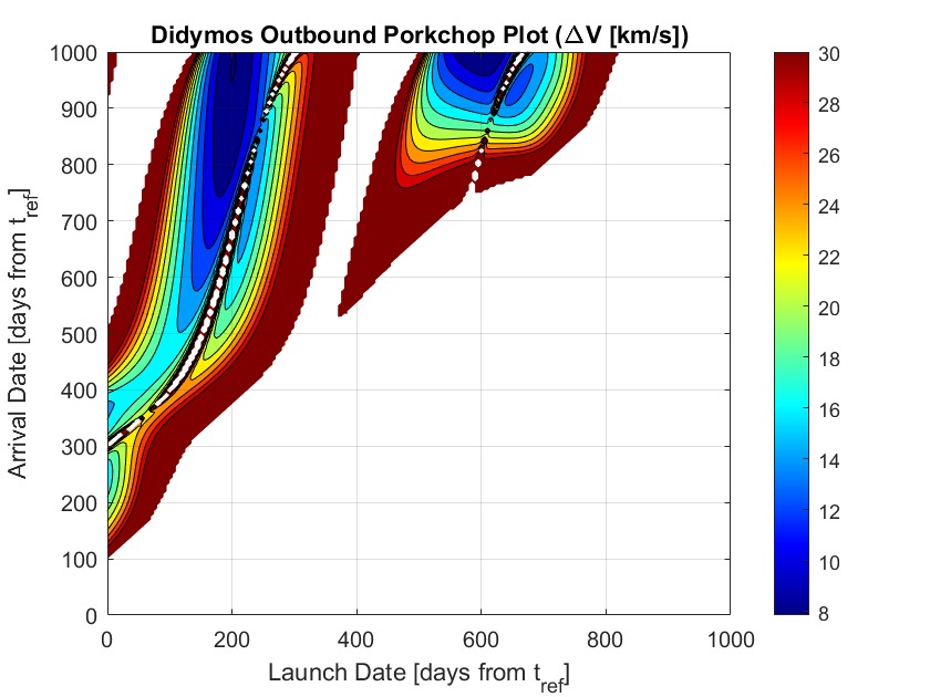
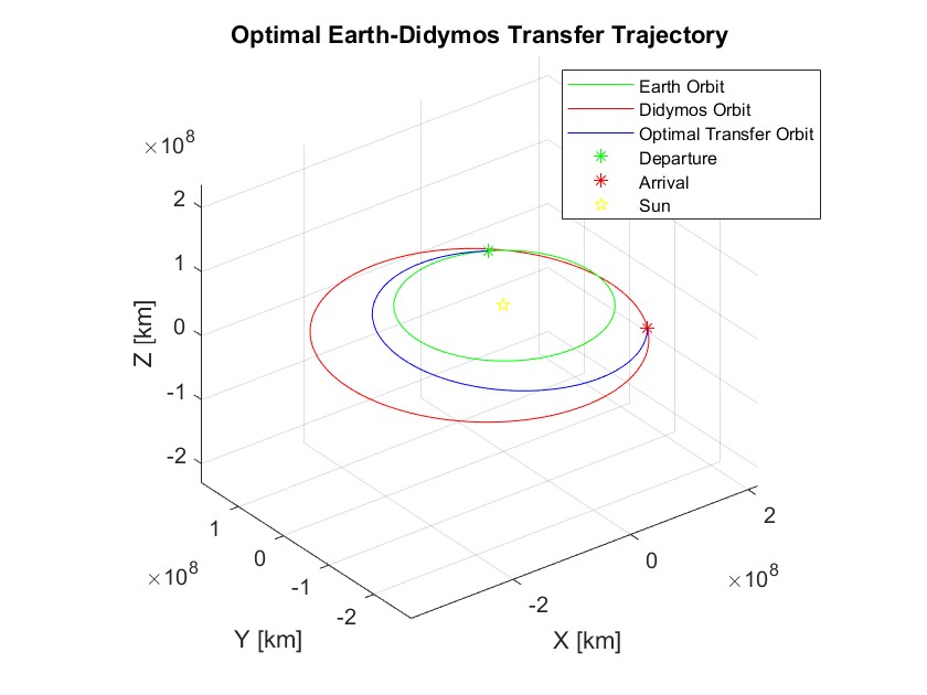
From reference orbital elements for Earth and Didymos, propagate each along its heliocentric ellipse — Earth to a launch date of tref + 12 days, Didymos to an arrival of tref + 412 days. Solve Lambert's problem for that 400-day transfer and take the total cost as ΔV = ‖v1 − vEarth‖ + ‖v2 − vDidymos‖, assuming a zero sphere of influence at each end. Then sweep launch and arrival dates on a 5-day grid from 0 to 1000 days (skipping transfers shorter than 100 days) to build a porkchop plot, and pick the cheapest departure/arrival pair out of it — the fixed 12-to-412-day transfer sits well outside the porkchop's low-cost trough.
%% Problem 4: Mission to Didymos
% Aras Vakilimafakheri
% Prof. Yuri Shimane
% MAE 146 - Astronautics
% Final Project

%% Given Constants:
clc;
clear;
close all;
format long;

AU = 149.6e6;   % [km]
MU = 132712000000;  % [km^3/s^2]
day = 86400;    % [s]

kep_earth = [1.00000011*AU;
             0.016710212;
             deg2rad(0.00005);
             deg2rad(-11.26064);
             deg2rad(102.94719);
             deg2rad(100.46435)];

kep_didymos = [1.6442*AU;
               0.38385;
               deg2rad(3.4079);
               deg2rad(73.196);
               deg2rad(319.321);
               deg2rad(195.0)];

%% (a) What are the position and velocity vectors of Earth on t = tref + 12 days?
% First compute the cartesian state of
% Earth at the reference time

cartesian_earth_ref = kep2rv(kep_earth, MU);

% Propogate the Earth cartesian state by 12 days

t_earth = 12*day;
cartesian_earth_12 = propagate_elliptical(cartesian_earth_ref, t_earth, MU);

% Extract velocity and position vector via matrix index

earth_pos_12 = cartesian_earth_12(1:3);
earth_velocity_12 = cartesian_earth_12(4:6);

disp('Earth position vector @ t = tref + 12 days [km]:')
disp(earth_pos_12')
disp('Earth velocity vector @ t = tref + 12 days [km/s]:')
disp(earth_velocity_12')

%% (b) What are the position and velocity vectors of Didymos on t = tref + 412 days?

% First compute the cartesian state of
% Didymos at the reference time

cartesian_didymos_ref = kep2rv(kep_didymos, MU);

% Propogate the Didymos cartesian state by 412 days

t_didymos = 412*day;
cartesian_didymos_412 = propagate_elliptical(cartesian_didymos_ref, t_didymos, MU);

% Extract velocity and position vector via matrix index

didymos_pos_412 = cartesian_didymos_412(1:3);
didymos_velocity_412 = cartesian_didymos_412(4:6);

disp('Didymos position vector @ t = tref + 412 days [km]:')
disp(didymos_pos_412')

disp('Didymos velocity vector @ t = tref + 412 days [km/s]:')
disp(didymos_velocity_412')

%% (c) Earth to Didymos Transfer Cost
% Compute time of flight

departure = 12*day;
arrival = 412*day;
tof = arrival - departure;

% Lambert solver parameters

cw = 0;
eps = 1e-8;
tol = 1e-10;

% Solve Lambert's problem

[v1_lambert, v2_lambert, residual] = lambert_universal(earth_pos_12, didymos_pos_412, tof, MU, cw, eps, tol);

% Compute cost requirements

delta_v_earth = norm(v1_lambert - earth_velocity_12);
delta_v_didymos = norm(v2_lambert - didymos_velocity_412);

total_delta_v = delta_v_earth + delta_v_didymos;

disp('Total mission cost [km/s]:')
disp(total_delta_v')

figure;
hold on;
grid on;
axis equal;
xlabel('X [km]')
ylabel('Y [km]')
zlabel('Z [km]')
title('Earth to Didymos Transfer')

% Plot Earth orbit
ta_vals = linspace(0, 2*pi, 300);
earth_orbit = zeros(3, length(ta_vals));

% Generate for loop to plot many points on orbit so curve is smooth
for k = 1:length(ta_vals)
    kep_temp = kep_earth;
    kep_temp(6) = ta_vals(k);
    rv_temp = kep2rv(kep_temp, MU);
    earth_orbit(:,k) = rv_temp(1:3);
end

plot3(earth_orbit(1,:), earth_orbit(2,:), earth_orbit(3,:), 'g')

% Plot Didymos orbit
didymos_orbit = zeros(3, length(ta_vals));

% Generate for loop to plot many points on orbit so curve is smooth
for k = 1:length(ta_vals)
    kep_temp = kep_didymos;
    kep_temp(6) = ta_vals(k);
    rv_temp = kep2rv(kep_temp, MU);
    didymos_orbit(:,k) = rv_temp(1:3);
end

plot3(didymos_orbit(1,:), didymos_orbit(2,:), didymos_orbit(3,:), 'r')

% Plot transfer trajectory
% Builds the initial Cartesian state of the spacecraft transfer
cartesian_transfer_0 = [earth_pos_12; v1_lambert];
transfer_traj = zeros(3, 300);

for k = 1:300
    t_now = (k-1)/(300-1) * tof;
    rv_now = propagate_elliptical(cartesian_transfer_0, t_now, MU);
    transfer_traj(:,k) = rv_now(1:3);
end

plot3(transfer_traj(1,:), transfer_traj(2,:), transfer_traj(3,:), 'b')

% Mark departure and arrival points
plot3(earth_pos_12(1), earth_pos_12(2), earth_pos_12(3), 'g*')
plot3(didymos_pos_412(1), didymos_pos_412(2), didymos_pos_412(3), 'r*')

% Plot sun
plot3(0, 0, 0, 'ypentagram')

legend('Earth Orbit', 'Didymos Orbit', 'Transfer Orbit', 'Earth Departure', 'Didymos Arrival', 'Sun', 'FontSize', 8)

% Make graph 3D
view(3)

%% (d) Porkchop Plot
t_days = 0:5:1000;
DV_map = nan(length(t_days), length(t_days));

for i = 1:length(t_days)     % Launch Date (t0)
    t0 = t_days(i) * day;
    cartesian_earth_depart = propagate_elliptical(cartesian_earth_ref, t0, MU);
    for j = 1:length(t_days) % Arrival Date (tf)
        tf = t_days(j) * day;
        tof = tf - t0;
        if tof >= 100 * day
            cartesian_didymos_arrive = propagate_elliptical(cartesian_didymos_ref, tf, MU);
            try
                [v1_p, v2_p, ~] = lambert_universal(cartesian_earth_depart(1:3), cartesian_didymos_arrive(1:3), tof, MU, 0, 1e-10, 1e-4);
                dv = norm(v1_p - cartesian_earth_depart(4:6)) + norm(v2_p - cartesian_didymos_arrive(4:6));
                if dv < 50 % Filter out unphysical outliers
                    DV_map(j, i) = dv;
                end
            catch
                continue; % Skip failed convergences
            end
        end
    end
end
figure(2);
contourf(t_days, t_days, DV_map, 0:2:30);
colorbar; colormap('jet'); grid on;
xlabel('Launch Date [days from t_{ref}]'); ylabel('Arrival Date [days from t_{ref}]');
title('Didymos Outbound Porkchop Plot (\DeltaV [km/s])');

%% (e) Optimal Trajectory Visualization
% Find minimum delta V point from the porkchop plot
[min_dv, linear_idx] = min(DV_map(:), [], 'omitnan');
[row, col] = ind2sub(size(DV_map), linear_idx);

best_t0_days = t_days(col);
best_tf_days = t_days(row);
best_tof = (best_tf_days - best_t0_days) * day;

fprintf('Local Minimum Found:\n');
fprintf(' Launch Date: t_ref + %.0f days\n', best_t0_days);
fprintf(' Arrival Date: t_ref + %.0f days\n', best_tf_days);
fprintf(' Minimum Delta-V: %.4f km/s\n', min_dv);

% Recalculate best transfer
cartesian_earth_opt = propagate_elliptical(cartesian_earth_ref, best_t0_days * day, MU);
cartesian_didymos_opt = propagate_elliptical(cartesian_didymos_ref, best_tf_days * day, MU);

earth_pos_opt = cartesian_earth_opt(1:3);
earth_velocity_opt = cartesian_earth_opt(4:6);

didymos_pos_opt = cartesian_didymos_opt(1:3);
didymos_velocity_opt = cartesian_didymos_opt(4:6);

[v1_opt, v2_opt, residual_opt] = lambert_universal(earth_pos_opt, didymos_pos_opt, best_tof, MU, cw, eps, tol);

delta_v_earth_opt = norm(v1_opt - earth_velocity_opt);
delta_v_didymos_opt = norm(v2_opt - didymos_velocity_opt);
total_delta_v_opt = delta_v_earth_opt + delta_v_didymos_opt;

fprintf(' Recomputed Total Delta-V: %.4f km/s\n', total_delta_v_opt);
fprintf(' Lambert Residual: %.4e\n', residual_opt);

figure(3);
hold on;
grid on;
axis equal;
xlabel('X [km]');
ylabel('Y [km]');
zlabel('Z [km]');
title('Optimal Earth-Didymos Transfer Trajectory');

% Plot Earth orbit
ta_vals = linspace(0, 2*pi, 300);
earth_orbit = zeros(3, length(ta_vals));

for k = 1:length(ta_vals)
    kep_temp = kep_earth;
    kep_temp(6) = ta_vals(k);
    rv_temp = kep2rv(kep_temp, MU);
    earth_orbit(:,k) = rv_temp(1:3);
end

plot3(earth_orbit(1,:), earth_orbit(2,:), earth_orbit(3,:), 'g')

% Plot Didymos orbit
didymos_orbit = zeros(3, length(ta_vals));

for k = 1:length(ta_vals)
    kep_temp = kep_didymos;
    kep_temp(6) = ta_vals(k);
    rv_temp = kep2rv(kep_temp, MU);
    didymos_orbit(:,k) = rv_temp(1:3);
end

plot3(didymos_orbit(1,:), didymos_orbit(2,:), didymos_orbit(3,:), 'r')

% Plot optimal transfer trajectory
cartesian_transfer_opt = [earth_pos_opt; v1_opt];
transfer_traj = zeros(3, 300);

for k = 1:300
    t_now = (k-1)/(300-1) * best_tof;
    rv_now = propagate_elliptical(cartesian_transfer_opt, t_now, MU);
    transfer_traj(:,k) = rv_now(1:3);
end

plot3(transfer_traj(1,:), transfer_traj(2,:), transfer_traj(3,:), 'b')

% Mark departure and arrival points
plot3(earth_pos_opt(1), earth_pos_opt(2), earth_pos_opt(3), 'g*')
plot3(didymos_pos_opt(1), didymos_pos_opt(2), didymos_pos_opt(3), 'r*')

% Plot Sun
plot3(0, 0, 0, 'ypentagram')

legend('Earth Orbit', 'Didymos Orbit', 'Optimal Transfer Orbit', ...
       'Departure', 'Arrival', 'Sun', 'FontSize', 8)

view(3)